
Email Us 351proj@gmail.com

About the Project
The purpose of our project is to create a Japanese/English Language Identifier using techniques learned in our EECS 351 (Introduction to Digital Signal Processing) course and a few techniques outside of the classroom. Of course, the goal along the way is to learn to apply DSP in real-world projects outside of purely theoretical manipulations.
We chose this project because it coincided both with our personal interests and held contemporary value. From a real-world standpoint, because people and cultures are becoming increasingly interconnected in an ever-shrinking world, the value of an accurate universal translator is rising exponentially. Our project is essentially the first component of such a device: a universal language classifier/identifier.
Our belief is that, once we develop a robust procedure for distinguishing Japanese and English, it should be relatively straightforward to include support for other languages as many of the same techniques should still be usable across other languages.
Prologue

Lesson 3
Lesson 2
Lesson 1
01
02
03
What We've Learned
Epilogue
Fourier transforms are potentially a viable method of classification (but not the way we did it). In our setup, we used all N coefficients of an extremely long speech sample (4 - 18 seconds). To improve Fourier transform analysis, we think we need to analyze shorter speech segments and disregard the first coefficient because shorter segments help show frequency content with respect to time and the first coefficient is simply average power.It requires short speech segments to properly represent the spectral quantities of a spoken sound. Additional processing of this nature would lead to the Mel-frequency Cepstrum Coefficients, which is why we think this is a way to improve FFT analysis.
Our assumption that every phoneme had a relatively unique time-domain waveform was flawed. And this, in turn, invalidated much of our cross-correlation data. To improve this method, we would need to ensure that waveforms (both the sample and sound to be cross-correlated with) have the same amplitude and analyze the output based on the shape of the waveforms. In the context of speech analysis, this is nearly impossible to implement as it would require "perfect" speech samples, a very subjective thing.
The neural network is an extremely powerful model capable of representing complex models with just a mass of simple scalar operations. Naive Bayes definitely has potential, but compared to neural networks it may simply just not be enough to solve a classification problem with features that seem to be neither normally nor multinomially distributed.
Step 4 - Results & Conclusions
The Process
FFT w/ Naive Bayes
After our initial qualitative analysis of the FFT, we used the coefficients of the discrete Fourier transform as features in a Naive Bayes model. Overall, we had very poor results with the Bayes classifier. But as expected, assuming an mvmn distribution did give us better results as compared to assuming a normal distribution. As seen below, when assuming a normal distribution, the predictor was heavily skewed towards English.
During our first progress report, the normal distribution was actually skewed towards Japanese. The only thing that had changed since then were our training files, which we increased from around 25 to around 75. Since the normal distribution is easily influenced by mean and variance, a small change in training files completely changes the bias of this predictor, which is a reason why we did not continue to use it for FFT analysis.
After increasing the number of training files, the performance of the Naive Bayes classifier improved, but not enough to be usable. A 62.5% accuracy is only slightly better than a coin toss, and this would not be enough to make a reliable classifier.
Something we realized afterwards was that, similarly to mel-frequency cepstral coefficients, DFT coefficients of long audio samples are not really representative of much, since in a long sequence of speech many different frequencies will likely be covered. For this to have been more accurate, we should have tried segmenting into short samples like we did for the MFCCs.
Cross-correlation with Naive Bayes
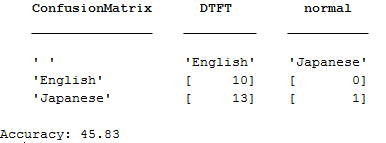
After passing in Japanese vowels and English consonants to cross-correlate with the training files, we accumulate data such as peak numbers and peak frequency. Using these data points, we created a table to use in a supervised Naive Bayes classifier. We find that the accuracy is fairly low even after changing the training files and distribution types. The results can be seen below:
An interesting observation that we've noted is that the mistakes always lean towards one language. This leads us to consider that the data input for training perhaps is not statistically different enough to be used for classification purposes. Examples can be seen below.
After further research and analysis of this method, we discovered that cross-correlation was not behaving as we had expected it to. In our approach, we had assumed that each sound had a unique and easily distinguishable time waveform that could easily be identified through cross-correlation. However, it turns out that cross-correlation in program was also producing phenomenal peaks in samples that for sure did not have the sound we were correlating with. Because we discovered this just a week before the conclusion of the term, we resigned ourselves to the fact that our cross-correlation scheme was flawed and cut short our efforts for extracting data from consonant cross-correlations. With time, we would have liked to further research and analyze cross-correlation speech data.
Mel-frequency Cepstral Coefficients (MFCCs) w/ Neural Network
After calculating the MFCCs for every single 25 ms segment out of our ~75 test files, we had over 63,000 vectors each containing 13 coefficients, about 27,000 of them English, and 36,000 Japanese. After training the neural network, we saw promising initial results.
As can be seen from the confusion matrix, there is an 87.3% success rate with classifying individual 25ms samples. Cross-validation through the form of repetitive retraining gives a consistent 85~88% accuracy. Likewise, the receiver operating characteristic plot shows great performance with the classification. To transition from the 25ms classification to classification of actual voice samples, we simply split the test file into 25ms segments and classified every segment with the neural network. If more segments were classified as English, then the voice sample was determined to be English, and vice versa. This showed great results with our test files.
As far as the tests go, the neural network exhibits 100% accuracy. Of course, we were cautious with these initial results, as there is no such thing as a perfect classification model. We retrained several times, but each time the confusion matrix ended up looking the same. This then brought us to a new question. MFCCs are an already established standard in speech analysis, so that was definitely a large contributing factor to this success. However, was the excellent performance of this model the work of the MFCC, or the neural network? We decided to try one more implementation to see.
MFCC w/ Naive Bayes
Which brings us back to our Naive Bayes classifier. We again tried both normal and mvmn distributions, to see the following results.
Contrary to the FFT Naive Bayes model, MFCC actually has better performance with a normal distribution. The mvmn distribution produces disappointing results, hovering around 50%. The normal distribution gives 75%, which is much better, but still nothing compared to the Neural Network model. One main contributing factor is, again, perhaps the independence assumption. Simple probabilistic classifiers probably just aren't enough to model the differences between two languages.


Confusion Matrix and Receiver Operating Characteristic of the neural network model. In the confusion matrix, 1 is English and 2 is Japanese


Results assuming data is normally distributed. Accuracy decreases with increasing number of training files
Results assuming data is multivariate multinomially distributed. Accuracy is low


Classifier assuming data is normally distributed. Results are heavily skewed towards classifying one language. It is always accurate in one language.
After meeting with Professor Balzano and learning more about certain speech processing techniques, we decided to proceed with three different classification methods. The first one--based on recommendation--involved feeding FFT coefficients into the Naive Bayes built-in MATLAB model. The second method involved cross-correlating our speech samples with certain sounds specific to only one language; the existence or nonexistence of a sound would help us decide whether a sample was English or Japanese. The third method involved determining mel-frequency cepstrum coefficients and feeding them into 1) a Naive Bayes Model and 2) a neural network.
Fast Fourier Transform (FFT)
The Discrete Fourier Transform (DFT) is a variation of the Fourier transform. Since sounds are essentially vibrations, the Fourier transform is highly valued to easily map and analyze frequency. All analysis is done on finite sound samples thus the DFT is used. The DFT converts equally spaced samples of a function in the time domain and converts them into equally spaced samples of a complex-valued function in the frequency domain. The DFT equation can be seen below:
The FFT is an algorithm that computes the DFT but hastens the calculation by decomposing the DFT matrix into mostly zero factors. This simplifies the DFT complexity from O(n^2) to O(n log(n)). This can be summarized below:
DFT:
Split equation into odd (2r+1) and evens (2r) and simplify:
Flow Diagram:
Proof and diagram taken from Professor Balzano's Lecture 10 FFT Computation PDF
Note: N-Point DFT and FFT transforms can be taken by using a user defined N instead of N number of discrete samples from the time domain function.
Cross-Correlation
Cross-correlation is a technique for measuring the similarity of two functions as a function of displacement relative to one another. This can be used for analyzing how similar two waveforms are to each other. Analysis is done in the time domain. The equation definition and graphical representation can be seen below:
Equation:
Graphical Representation:
Graphical repesentation taken and edited from https://en.wikipedia.org/wiki/Cross-correlation
Mel-Frequency Cepstral Coefficients (MFCC)
MFCCs are representations of short-term power on the Mel scale of frequency. The Mel scale relates the pitch of a tone to the actual measured frequency. Human ears are better at hearing change in low frequencies than high frequencies and this scale matches that. The conversion can be seen below:
MFCCs are used to represent human speech patterns and can differentiate between different phonemes (different sounds of a language). MFCC are very commonly used in speech recognition. The steps to generating the MFCC are below:
-
Take the DFT of short frames (20-40ms) with some overlap (~10ms)
-
Estimate the power spectrum of each frame through periodogram estimation
-
Apply Mel filterbank to the power spectrum and sum the energy
-
Take the logarithm
-
Take the discrete cosine transform (DCT)
-
Keep coefficients 2-13
Reasoning:
-
The signal must be separated into small frames since statistically stationary data is more reliable.
-
Power spectrum is used because the human cochlea reacts depending on the spectrum
-
Map to a Mel scale since it is a better representation of perceived frequency
-
Take the logarithm since hearing is on a log scale
-
Take DCT to decorrelate data
-
Take coefficients 2-13 since coefficient 1 is overall power (not helpful), and other points are superfluous
For our classifiers we looked at two main algorithms: Naive Bayes and artificial neural networks.
Naive Bayes
The Naive Bayes algorithm is a classification method that assumes the existence of a particular
feature in a class is independent of any other feature in the same class. Bayes' Theorem is used
to calculate conditional probabilities of an event based on known information of the conditions
that may be related to it. The probability of some input belonging in class C among K possible outcomes
Step 2 -Choosing Classifiers
The Process

can be written as: , where x is a vector representing n independent features, and Z is a constant scaling factor dependent on the features. To determine what class some input data actually belongs to, the Bayes classifier picks the class that is the most probable. Simply put, it finds the conditional probabilities of the data
belonging to each of the classes C_1...C_k, given knowledge of supposedly independent
features {x}, and then picks the class for which the probability is highest.
To actually determine the conditional probabilities of the features, we need to define a distribution for the data. The two distributions that we used in our Naive Bayes classifier were the normal Gaussian distribution and the multivariate multinomial (mvmn) distribution.
With the normal distribution, we simply assume that the values of the features are normal within each class. Separating the data for the predictors by class, we can calculate the value for the mean and variance of the feature within the class, then build a normal distribution based on those 2 features.
With multinomial distributions, a feature vector x=(x1,...,xn) describes frequencies of events, with x_i representing the number of times event i happened when event C occurs. This is a distribution model more commonly used for grouping classification, and thus the type of distribution we initially expected to be better.
Formulas from en.wikipedia.org/wiki/Naive_Bayes_classifier


Artificial Neural Network
Neural Networks are composed of layers of nodes which are interconnected; data is put into the network from the input layer, which passes through to the hidden layer where the data is processed with a network of weighted connections. After the processing is done, the hidden layer sends the data through to the output layer which tells the user the final answer. The goal of this algorithm, as its name implies, is to simulate the way the human brain works. As such, we train a neural network in much the same way we teach people: by showing examples (inputs) and telling them what it is (output).
In the single-layer neural network we used, we implemented a backpropagational neural network known as the delta rule. Each time the network is given an input pattern, also known as an epoch, it propagates forward through the network and generates output activations for the nodes it passes through before arriving at the output layer. The target of the same input data (the class we know the input data belongs to) is propagated backwards through the same nodes and calculates the deltas of all the neurons. These deltas can then be used to update the weighed connections between the nodes. Put very simply, the neural network first makes a random guess as to what an input pattern is, then checks to see how far away its prediction was from the actual class and makes adjustments to the weights of the connections. Clearly, the goal is to feed the neural networks enough information so it can make more and more accurate predictions.
Neural networks can be used to model many different types of data patterns due to its complex nature, but the backpropagation makes training much slower as the network size increases. For the purposes of this project though, we were able to get away with just using one hidden layer of 10 nodes.


A representation of a multi-layered neural network. Courtesy of M. Dehghani, M. Eghtesad, A. A. Safavi, A. Khayatian and M. Ahmadi (2008). Neural Network Solutions for Forward Kinematics Problem of HEXA Parallel Robot, Parallel Manipulators, New Developments, Jee-Hwan Ryu (Ed.), InTech, DOI: 10.5772/5374.


Step 1 - Data Acquisition
The Process
The first step to creating our language classifier was simple: we had to find English and Japanese sound files. The key idea we set out with during this step was making sure our sample space was both realistic--so that it accurately described contemporary speech--and simple to analyze--so that our classification schemes didn't require skills way beyond our EECS 351 background. We decided to do this by having samples by multiple speakers for both languages and having male and female speakers.
We downloaded our English files from tatoeba.org and our Japanese files from voicetext.jp and voice-koesen.com. Unfortunately, we did not manage to get 50/50 male-female samples. The English sample set was skewed towards male samples, and the Japanese sample set was skewed towards female samples.

Language Identification Program
Techniques in the Time and Frequency Domains
Allen Du, Calvin Shih, Saad Khatri
Hi! Thanks for visiting our EECS 351 Project website. The purpose of this site is to offer a dedicated place for us to introduce our project, illustrate how we designed and implemented it, and highlight what we learned from it. We've also added some of our in-progress works in two of the above tabs: Progress Report and Project Presentation.

Step 3 - Implementing Classifiers
FFT Analysis w/ Naive Bayes
For this implementation, we simply used DFT coefficients as features in a Naive Bayes classifier. Although the independence assumption may not hold for these features, Naive Bayes is known to function relatively well even in such scenarios. We did tests with both normal and multivariate multinomial distributions of predictors, then made some simple confusion matrices to interpret our results. The only other factor here is the number of coefficients we choose to use. For the most part, we stuck with powers of 2 under 10000 (1024,2048,4096...) since MATLAB calculates N-point FFTs of powers of 2 slightly faster.
Cross-Correlation
To use cross-correlation, we pulled open some unique features of the English and Japanese language (see Progress Report). We cross-correlated our training files with Japanese vowel sounds and English consonant sounds, then used an envelope to define the peaks of the resulting waveforms to try to see where and how often there was a great amount of similarity. We then extracted a simple statistics, peaks per second, to see if our Naive Bayes model could use these as probabilistic classifiers.
MFCC w/ Naive Bayes
For MFCC's, we split the audio samples into tiny 25 ms segments, with 10 ms of overlap between each new segment, because MFCC's are only meaningful when applied to short segments of speech. We calculate 13 coefficients total, not counting the first. The first MFCC coefficient is generally representative of the volume of the clip, which is not relevant to language classification applications, and any more coefficients do not provide much extra information. For the Naive Bayes classifier, we used the individual MFCC coefficients as features and tried both normal and mvmn distributions.
MFCCs w/ Neural Network
After calculating the MFCCs, we use MATLAB's Neural Network Toolbox to train a new model. Similar to the Naive Bayes model, we pass in a large matrix with each column being a different MFCC and each row being a new 25 ms segment of audio. After telling MATLAB which columns belong to English voice files and which Japanese, it can start training the model as described in the previous section. The Neural Network Toolbox randomly selects 15% of the samples to use as test samples, so only 85% of the samples we actually feed MATLAB are actually used to train the model. This means that we can retrain the model and get slightly different results allowing us to cross-validate with ease. After the training is done, we can generate a function that simulates the Neural Network, since in the end it is just a network of weighted scalar connections, easily rewritten as many matrix functions.